Broteína: Self-Distillation Unlocks Few-Step Protein Design
How teacher-score alignment changes the few-step search frontier in in silico protein backbone generation.
May 31, 2026 · 21 min read
TL;DR
Under the reported in silico benchmarks, Broteína establishes a new search-efficiency frontier among the Proteína and DPBG-style systems compared here. In the 500-sample unconditional evaluation, \(\mathcal{B}^{1}\) reaches the lowest effective NFE per designable backbone and per designable cluster, while native \(\mathcal{B}^{16}\) is the strongest few-step row when classic search metrics and the reported distributional metrics are considered jointly. On full-30 MotifBench, aligned students also find more unique solutions per backbone-generation NFE than the matched-step, author-implemented DPBG-style baselines.
Most notably, the compressed students do more than recover the base model's search yield. The selected 5-step, 8-step, and native 16-step operating points reach 339, 361, and 354 designable clusters, respectively, all above the 400-step low-temperature Proteína reference's 297. The 8-step student finds 64 more clusters, an improvement of about 22%, while using 50× fewer sampling steps. To our knowledge, 361 is the highest designable-cluster count reported under this standard five-length, 500-sample protocol.
The principal methodological contribution is not a new backbone architecture or a new distillation objective. Broteína changes the distribution being distilled: it first fine-tunes the teacher so its native \(\gamma = 1\) score field targets the useful low-temperature design distribution, then distills that aligned teacher into few-step generators.
Part I
Protein Design Is Search
Backbones Are Structural Hypotheses
A backbone generator does not output a complete protein. It outputs the 3D trace of a protein chain before the amino-acid sequence is chosen. To turn that structure into a candidate, the usual computational loop is inverse folding and refolding: design sequences for the backbone, predict whether those sequences fold back to the intended shape, then keep the structures that survive.
In the evaluations here, ProteinMPNN proposes sequences, ESMFold folds them, and a backbone is counted as designable if the folded structure is within 2.0 Å Cα-RMSD of the generated backbone [6], [7]. This is not a perfect proxy for experimental success. It is biased by ProteinMPNN, ESMFold, the number of sequence attempts, and the RMSD cutoff. But it is an operationally meaningful proxy: if a generated backbone cannot pass this loop, it is not useful for this design workflow.
The Search Metric Is Not Just Designability
Designability answers: what fraction of samples survive the realization pipeline?
Search asks a stronger question: how many distinct realized candidates did we get for the compute we spent?
This is why designable clusters are central. We cluster only the designable structures, so the metric combines realization rate and fold-level coverage. A model with 98% designability but a narrow set of repeated folds can be less useful than a model with slightly lower designability and many more distinct realized clusters.
The compute side is counted in neural function evaluations, or NFEs. For these samplers, one sampling step is one network call, so a \(K\)-step generator spends \(K\) NFEs per candidate. Two useful efficiency summaries are:
\[ \mathrm{Eff.\ NFE}_{\mathrm{designable}} = \frac{K}{\mathrm{designability}}, \qquad \mathrm{NFE/cluster} = \frac{500K}{\#\mathrm{designable\ clusters}}. \]
The first asks how many backbone-generator calls are needed, in expectation, to get one designable backbone. The second asks how many such calls were spent per distinct designable cluster in the 500-sample classic evaluation. These metrics isolate generation cost: they exclude ProteinMPNN sequence design, ESMFold refolding, clustering, experimental validation, and total wall-clock cost.
Part II
Preliminaries: Scores, Temperature, And Distillation
Why Iterative Generation Is Expensive
Diffusion and flow protein generators repeatedly call a neural network to move noise toward a backbone [4], [5]. Proteína uses 400 sampling steps, while large-scale Genie 2 evaluations use 1000 [1], [9]. Each backbone then enters sequence design, refolding, scoring, and clustering, so reducing neural function evaluations expands the searchable space under a fixed budget.
The goal is to replace hundreds of calls with 1, 5, 8, or 16 while preserving the reported designable-search frontier.
From Flow Fields To Scores
Proteína parameterizes a velocity field \(v_\theta(x_t,t)\). Distribution-matching distillation is written in terms of the score
\[ s_t(x_t)=\nabla_{x_t}\log p_t(x_t), \]
which points toward higher density at noise level \(t\). For the Gaussian path used here, velocity gives an approximate score:
\[ s_\theta(x_t,t)\approx\frac{t\,v_\theta(x_t,t)-x_t}{1-t}. \]
This bridge lets score-based distillation operate on a flow model [1].
Temperature Changes The Deployed Distribution
The sampling scale \(\gamma\) controls stochasticity. Native sampling uses \(\gamma=1\); lowering it often raises designability but can collapse coverage. In the base model, moving from \(\gamma=1\) to \(0.55\) raises designability from 6.6% to 83.2% and clusters from 29 to 277. Cooling further to \(0.35\) raises designability to 97.2% but reduces clusters to 226.
Low temperature is thus not a harmless inference knob. It creates the distribution that practitioners actually use, and that distinction matters when the model is distilled.
What Distribution Matching Learns
SiD-style distillation uses a fixed teacher, a fast generator, and an auxiliary model that estimates the student's score. Their score difference moves the generated distribution toward the teacher [3]. DPBG adapts this idea to protein backbones [2].
More details.
There are three learned objects in the distillation loop: a fixed teacher \(\mathcal{T}_\phi\) with score \(S_\phi(x_t,t)\), a few-step generator \(G_\theta\) that produces \(x_g\), and an auxiliary score model \(\mathcal{A}_\psi\) with score \(S_\psi(x_t,t)\). The auxiliary model is needed because a one- or few-step generator does not directly provide a reliable score throughout noisy space. It is trained on noised student samples to estimate the score of the distribution that the student currently produces.
A raw Fisher-style score gap would compare \(S_\phi\) and \(S_\psi\), but that divergence alone is not a stable generator objective. The practical SiD signal also uses their difference as the direction for updating generated samples:
\[ \begin{aligned} \mathcal{L}_{\mathrm{SiD}}=\mathbb{E}_{x_g,t}\Big[&(1-\alpha)\frac{\omega(t)}{\sigma_t^4}\lVert S_\phi(x_t,t)-S_\psi(x_t,t)\rVert_2^2 \\ &+\frac{\omega(t)}{\sigma_t^4}(S_\phi-S_\psi)^\top(S_\psi-x_g)\Big]. \end{aligned} \]
The first term measures teacher-versus-student score mismatch through the auxiliary model; the second supplies the generator update direction. DPBG derives the corresponding flow-matching form used for Proteína-style backbones. The important point here is that both terms inherit whichever distribution the fixed teacher represents.
The catch is which teacher distribution supplies that score. Direct distillation sees the base model at native sampling, while the useful deployed search distribution is colder:
\[ \text{distillation target}\approx p_{\mathcal{M}}(\gamma=1), \qquad \text{deployed target}\approx p_{\mathcal{M}}(\gamma<1). \]
DPBG distills first and then cools the student. A one- or five-step trajectory leaves that correction little room to reshape the distribution. Broteína instead changes the native teacher score field before distillation; direct one-step DPBG finds only 2 designable clusters, while aligned students make the low-step regime useful.
Part III
Self-Align The Teacher Before Distilling
What Is Being Aligned
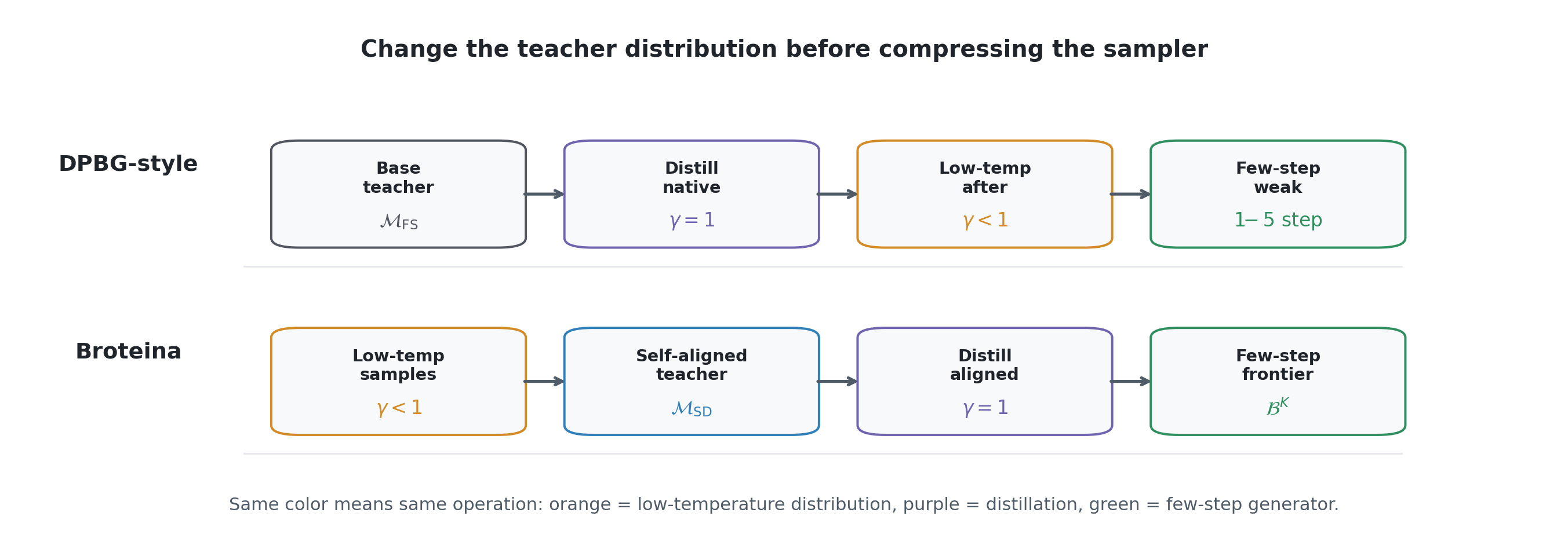
The alignment stage starts from \(\mathcal{M}_{\mathrm{FS}}^{\mathrm{no\text{-}tri}}\), the lighter Proteína model without triangle layers [1]. Synthetic alignment sets are generated from the useful low-temperature design distribution and then used to fine-tune the Proteína-style teacher with the normal flow-matching objective. The goal is not yet to make a fast model. The goal is to move the many-step teacher's native \(\gamma = 1\) score field.
Native \(\gamma = 1\) matters because this is the distribution the later distillation objective sees. If the aligned teacher only became useful after another low-temperature correction, the few-step student would inherit the same mismatch.
More details.
The schematic contrasts the distillation target, not the full training implementation. The DPBG-style path uses the native base teacher score as the distillation target and then relies on low-temperature sampling after distillation. Broteína changes the teacher distribution first, so the later score-distillation stage sees a native aligned teacher.
The unconditional experiments reported here use no self-conditioning. In Proteína, self-conditioning means the network receives an earlier clean-structure prediction as an additional input during sampling. That can improve some rows, but it changes the evaluation path and can change candidate rankings. The reported \(\mathcal{B}^{K}\) generators are therefore tied to the no-self-conditioning teacher-selection protocol.
The names used below are:
- \(\mathcal{M}_{\mathrm{FS}}^{\mathrm{no\text{-}tri}}\): base Proteína teacher.
- \(\mathcal{M}_{\mathrm{SD,C}}^{\mathrm{no\text{-}tri}}\): cluster-maximizing self-distilled teacher used for the reported unconditional few-step generators.
- \(\mathcal{M}_{\mathrm{SD,B}}^{\mathrm{no\text{-}tri}}\): balanced self-distilled alternative with stronger distributional fidelity.
- \(\mathcal{B}^{K}\): \(K\)-step Broteína generator distilled from the aligned teacher.
The Alignment Trajectory
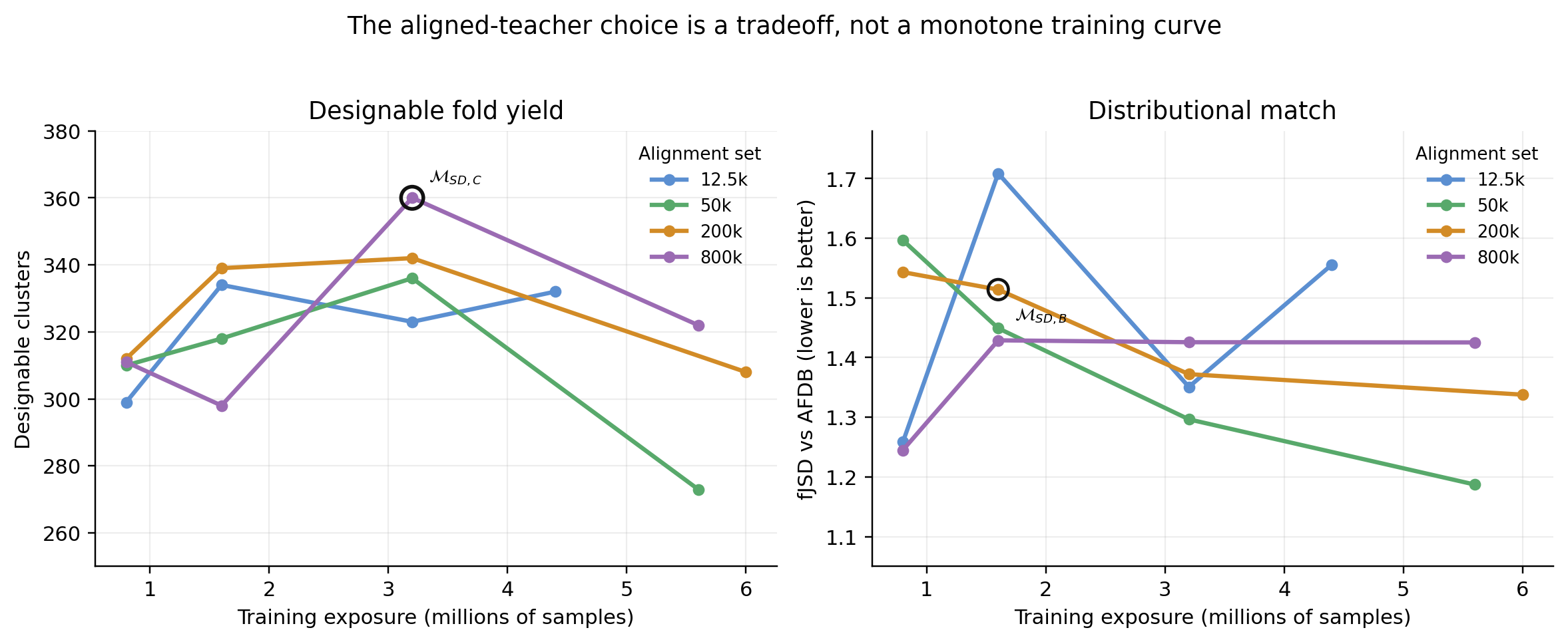
The teacher was selected from a 16-run grid over synthetic-set size and training exposure. Every candidate was evaluated at native \(\gamma=1\), without self-conditioning, to measure whether fine-tuning changed the teacher itself.
More details.
The grid tracks designability, cluster yield, diversity, secondary structure, FPSD, and fJSD. The reported students use \(\mathcal{M}_{\mathrm{SD,C}}^{\mathrm{no\text{-}tri}}\) because it has the highest native-sampling designable-cluster count in the 16-run grid: 360. \(\mathcal{M}_{\mathrm{SD,B}}^{\mathrm{no\text{-}tri}}\) is reported as a more distributionally faithful alternative, not as the student teacher. No checkpoint is uniformly best across every metric.
The base model gives 29 designable clusters at native sampling; the selected aligned teacher gives roughly 360. Checkpoint selection remains multi-objective because designability, cluster yield, diversity, and distributional match do not improve monotonically.
Why The Temperature Sweep Matters
The temperature sweep directly tests the self-alignment claim within the reported native-sampling evaluation. At \(\gamma = 1\), \(\mathcal{M}_{\mathrm{SD,C}}^{\mathrm{no\text{-}tri}}\) reaches 85.4% designability and 357 designable clusters; the base model requires lower temperature to become useful and peaks at fewer clusters in the same sweep.
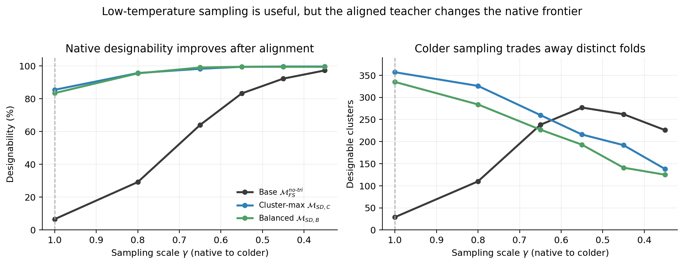
This observed shift supports the interpretation that alignment moves the teacher's native score field toward a more useful search distribution, reducing its reliance on an inference-time correction. The sweep establishes the change in behavior; it does not, by itself, identify a unique causal mechanism inside the network.
The sweep also tests a simpler explanation: that alignment merely substitutes one scalar temperature for another. If that were sufficient, colder sampling of the aligned teacher should continue improving its frontier. Instead, cluster yield falls from 357 at native sampling to 326 at \(\gamma = 0.8\), 260 at \(\gamma = 0.65\), and 138 at \(\gamma = 0.35\). This pattern is inconsistent with a simple scalar-temperature account, although it does not rule out other effects of fine-tuning.
The result is consistent with the training setup: alignment data are drawn from the useful low-temperature region where designability has largely saturated and diversity is beginning to narrow. A plausible interpretation is that fine-tuning transfers that region into the native sampler; confirming the internal mechanism would require additional causal analysis.
Part IV
Distill The Aligned Frontier
The Few-Step Search Frontier
After alignment, the student is no longer trained against the weak native base distribution. It is trained against a teacher whose native score field already searches designable regions.
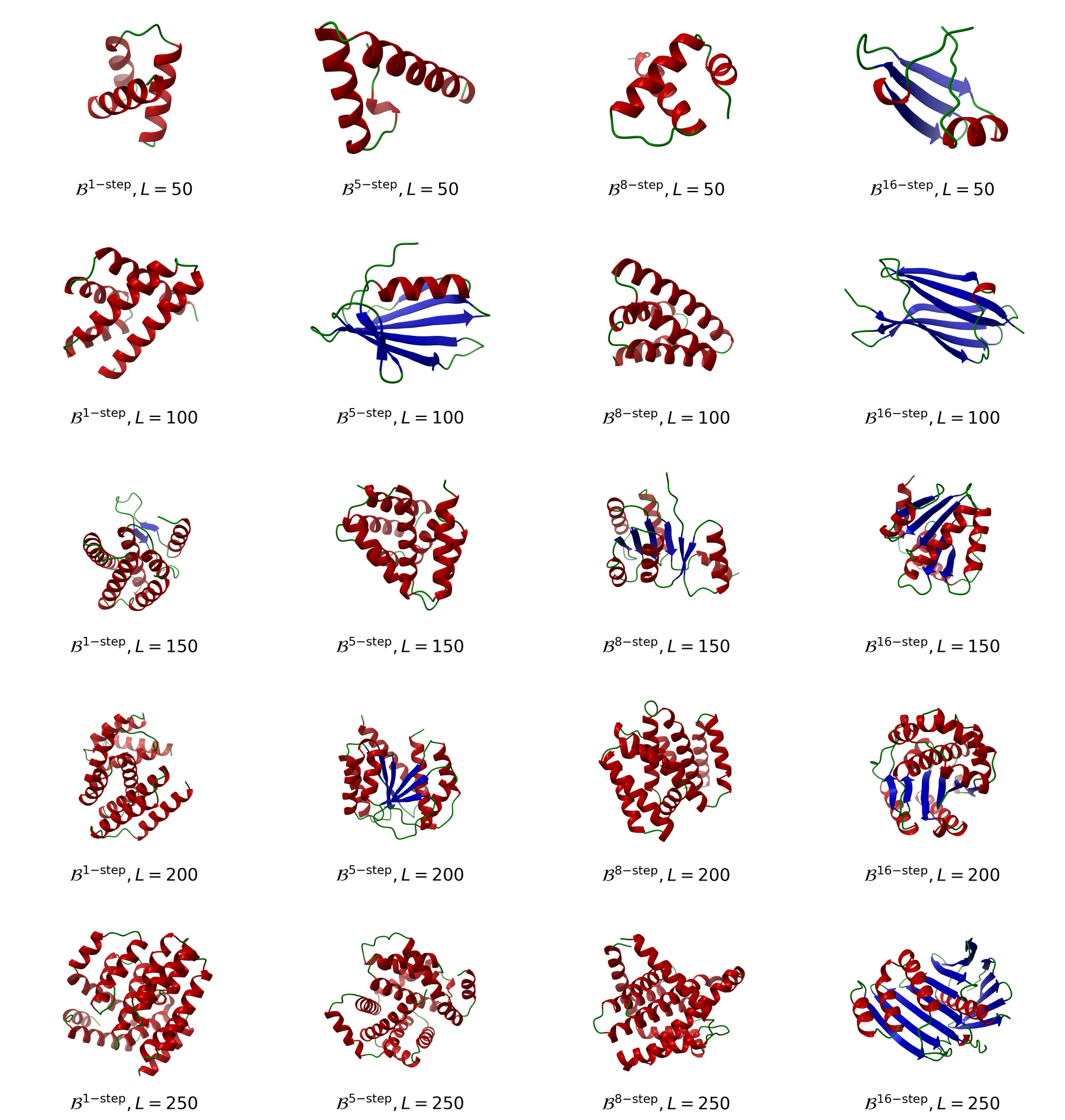
The length-wise view makes the search frontier easier to see. A useful few-step generator should not only do well at one chain length; it should keep finding designable, distinct structures across the 50, 100, 150, 200, and 250 residue evaluation grid.
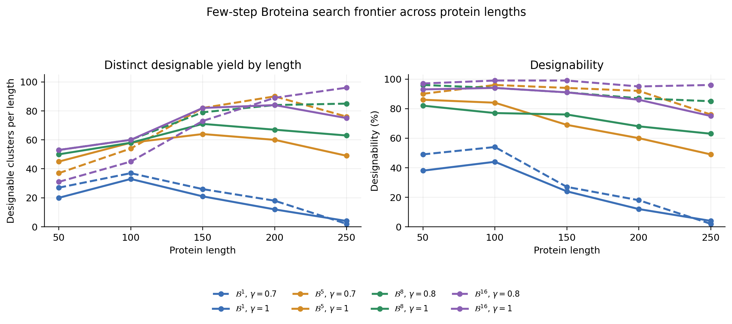
The table compares search yield, efficiency, and distributional fidelity.
| Model | \(\gamma\) | Des. ↑ | Cl. ↑ | Eff. NFE ↓ | NFE/cl. ↓ | Div. ↑ | \(\alpha/\beta\) | FPSD P/A ↓ | fJSD P/A ↓ |
|---|---|---|---|---|---|---|---|---|---|
| \(\mathcal{B}^{1\text{-}step}\) | 1.0 | 24.4% | 90 | 4.10 | 5.6 | 0.738 | 76.2/0.2 | 829/772 | 2.44/1.76 |
| \(\mathcal{B}^{1\text{-}step}\) | 0.7 | 30.0% | 110 | 3.33 | 4.5 | 0.733 | 76.8/0.2 | 860/797 | 2.63/1.89 |
| DPBG 1-step | 0.45 | 0.4% | 2 | 250.00 | 250.0 | 1.000 | 75.1/0.1 | 2470/2403 | 2.74/2.27 |
| \(\mathcal{B}^{5\text{-}step}\) | 1.0 | 69.6% | 276 | 7.18 | 9.1 | 0.793 | 74.6/2.1 | 413/396 | 2.70/1.90 |
| \(\mathcal{B}^{5\text{-}step}\) | 0.7 | 89.6% | 339 | 5.58 | 7.4 | 0.757 | 78.3/1.0 | 515/496 | 3.32/2.43 |
| DPBG 5-step | 0.45 | 47.4% | 151 | 10.55 | 16.6 | 0.640 | 71.5/0.0 | 457/424 | 3.48/2.54 |
| \(\mathcal{B}^{8\text{-}step}\) | 1.0 | 73.2% | 309 | 10.93 | 12.9 | 0.844 | 70.7/3.6 | 331/321 | 2.07/1.44 |
| \(\mathcal{B}^{8\text{-}step}\) | 0.8 | 90.6% | 361 | 8.83 | 11.1 | 0.797 | 74.4/2.7 | 447/432 | 2.76/1.96 |
| DPBG 8-step | 0.45 | 75.6% | 292 | 10.58 | 13.7 | 0.770 | 66.9/0.7 | 526/525 | 3.06/2.25 |
| \(\mathcal{B}^{16\text{-}step}\) | 1.0 | 87.8% | 354 | 18.22 | 22.6 | 0.806 | 70.7/5.4 | 305/310 | 1.74/1.23 |
| \(\mathcal{B}^{16\text{-}step}\) | 0.8 | 97.2% | 334 | 16.46 | 24.0 | 0.687 | 75.6/3.5 | 435/435 | 2.36/1.70 |
| DPBG 16-step | 0.45 | 94.4% | 287 | 16.95 | 27.9 | 0.610 | 63.2/4.6 | 404/394 | 1.94/1.54 |
| \(\mathcal{M}_{\mathrm{SD,C}}^{\mathrm{no\text{-}tri}}\) | 1.0 | 85.6% | 360 | 467.3 | 555.6 | 0.841 | 65.4/6.4 | 572/552 | 1.83/1.43 |
| \(\mathcal{M}_{\mathrm{FS}}^{\mathrm{no\text{-}tri}}\) | 0.45 | 94.2% | 297 | 424.6 | 673.4 | 0.630 | 64.4/4.6 | 317/291 | 1.80/1.24 |
More details.
The \(\mathcal{B}^{K}\) rows use the same five length buckets as the figure: 50, 100, 150, 200, and 250 residues, with 100 samples per length. The cluster totals are reported over that full five-length evaluation grid so the table and plot use the same evaluation convention.
Eff. NFE is \(K/\mathrm{designability}\), the expected number of network calls per designable sample. NFE/cl. is \(500K/\#\mathrm{clusters}\), the number of network calls spent per designable cluster in the 500-sample classic evaluation. FPSD and fJSD come from a separate 5,000-sample distributional evaluation.
The unconditional DPBG and base Proteína values are reference results transcribed from the benchmark comparison table rather than fresh reruns; the \(\mathcal{B}^{K}\) rows are Broteína evaluations on the stated five-length grid.
Within the unconditional rows shown, \(\mathcal{B}^{1}\) at \(\gamma = 0.7\) establishes the pure backbone-generation NFE frontier: 30.0% designability, 110 designable clusters, 3.33 effective NFEs per designable sample, and 4.5 NFEs per designable cluster. The reproduced DPBG one-step reference row reaches 0.4% designability, 2 clusters, and 250 effective NFEs per designable sample under its reported \(\gamma = 0.45\) setting.
Among the few-step student rows shown, \(\mathcal{B}^{8}\) at \(\gamma = 0.8\) has the highest designable-cluster yield: 361 clusters from 500 samples. That exceeds the 400-step low-temperature Proteína reference's 297 clusters by 64, or about 22%, while using 50× fewer sampling steps; it also narrowly exceeds the aligned 400-step teacher's 360. To our knowledge, 361 is the highest designable-cluster count reported under this standard five-length, 500-sample protocol. Its distributional metrics remain weaker than those of the native 16-step student, which is why the two rows represent different operating points.
Within this comparator set, the highlighted \(\mathcal{B}^{16}\) row at native \(\gamma = 1\) is the strongest overall few-step operating point when classic search metrics and distributional fidelity are considered jointly. It reaches 87.8% designability and 354 clusters, and improves over the reproduced DPBG 16-step row on cluster yield, diversity, NFE per cluster, FPSD, and fJSD. This is a multi-metric conclusion, not a claim of dominance on every column.
What Changed Relative To The Base Model
The direct empirical result is that self-alignment changes the teacher's native cluster-yield frontier in the reported in silico sweep, not only the speed of its students.
In the main 500-sample comparison, the 400-step low-temperature base reference reports 297 designable clusters. The selected 5-step, 8-step, and native 16-step students reach 339, 361, and 354 clusters, while the aligned teacher reaches 360 at native sampling. The students therefore do not merely preserve the base model under compression: several surpass its distinct designable yield with 25× to 80× fewer sampling steps. Together, these results support the interpretation that low-temperature sampling exposed a useful region that was difficult to compress from the native base teacher, and that alignment made this region easier for the student to copy.
Beyond Designability: A Surface-Cavity Case Study
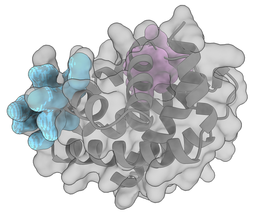
Designability asks whether designed sequences can be predicted to fold back to a generated backbone. It does not ask whether that backbone also exposes localized geometry that could be useful for downstream molecular design. To probe that second question, we revisited a representative designable scaffold from the one-step distilled generator, analyzed it with Fpocket, and visualized the result in ChimeraX [11], [12].
More details.
The scaffold is shown in gray with a semi-transparent molecular surface. The archived ICML analysis reports Pocket 7 with an Fpocket druggability score of 0.783, volume \(540.5~\text{\AA}^3\), polarity 8, and apolar proportion 0.796. Pocket 10 is reported with a druggability score of 0.682, volume \(347.8~\text{\AA}^3\), polarity 4, and apolar proportion 0.972. The original sample file and Fpocket output are no longer recoverable from the repository, so these are reported historical descriptors rather than a rerunnable benchmark.
The two detected cavities have meaningfully different geometric and compositional profiles: Pocket 7 is larger and contains more polar character, while Pocket 10 is smaller and more strongly apolar. This makes the one-step sample a concrete example of a designable generated scaffold with structured, chemically differentiated surface geometry, rather than only a favorable global fold metric. Such cavities are plausible starting points for downstream pocket- or ligand-oriented design, although this single historical example does not establish binding, biochemical function, or population-level pocket quality.
Part V
Motifs And Efficiency
Motif Scaffolding Is The Harder Search Problem
Unconditional generation asks for plausible, designable protein-like structures. Motif scaffolding adds a constraint: build a full backbone around a specified motif. This is closer to functional design because the motif may encode an active-site geometry, binding interface, or other structural requirement.
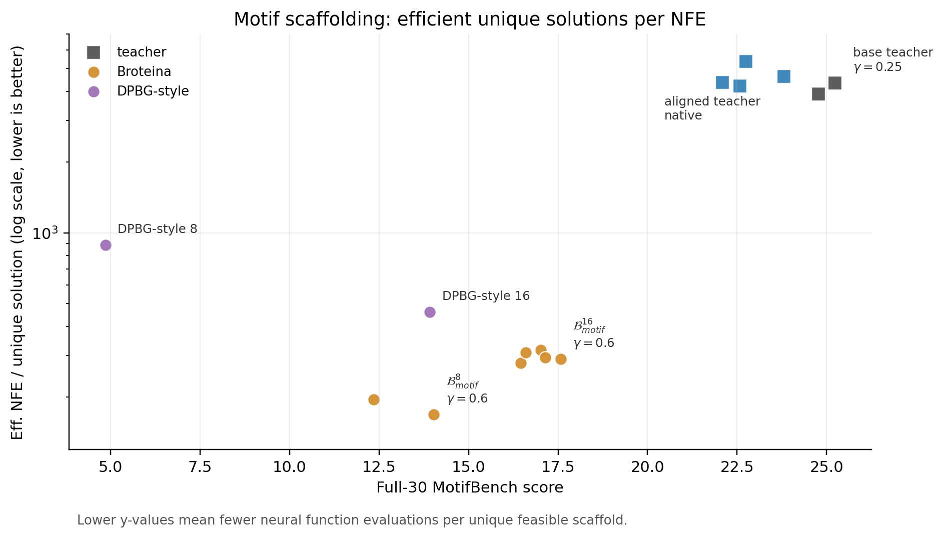
Proteína evaluated motif scaffolding on the RFdiffusion motif benchmark and recommends sampling around \(\gamma = 0.5\) [8], [1]; the evaluations below use the newer MotifBench protocol [10]. In the full-30 MotifBench sweep used here, \(\gamma = 0.25\) is the selected base-teacher operating point. The 400-step teachers remain stronger references on average MotifBench score; the frontier claim below concerns unique solutions and backbone-generation NFE, not average-score dominance.
The DPBG-style motif rows are author-implemented matched-step baselines that apply direct distillation to motif scaffolding; they are not motif results reported in DPBG. They isolate the effect of aligning the teacher before applying the same broad distill-then-cool strategy.
| Model | \(\gamma\) | Steps | MotifBench ↑ | Tasks ↑ | Unique ↑ | Successes ↑ | Eff. NFE/Unique Sol. ↓ |
|---|---|---|---|---|---|---|---|
| \(\mathcal{B}_{\mathrm{motif}}^{16}\) | 1.0 | 16 | 16.46 | 12 | 172 | 227 | 279 |
| \(\mathcal{B}_{\mathrm{motif}}^{16}\) | 0.6 | 16 | 17.57 | 12 | 165 | 255 | 291 |
| DPBG-style motif 16-step | 0.25 | 16 | 13.92 | 10 | 104 | 133 | 462 |
| \(\mathcal{B}_{\mathrm{motif}}^{8}\) | 1.0 | 8 | 12.35 | 11 | 123 | 158 | 195 |
| \(\mathcal{B}_{\mathrm{motif}}^{8}\) | 0.6 | 8 | 14.03 | 12 | 142 | 180 | 169 |
| DPBG-style motif 8-step | 0.25 | 8 | 4.85 | 6 | 27 | 46 | 889 |
| \(\mathcal{M}_{\mathrm{SD}}^{\mathrm{motif}}\) | 1.0 | 400 | 22.09 | 16 | 275 | 320 | 4,364 |
| \(\mathcal{M}_{\mathrm{SD}}^{\mathrm{motif}}\) | 0.6 | 400 | 23.81 | 14 | 259 | 423 | 4,633 |
| \(\mathcal{M}_{\mathrm{FS}}^{\mathrm{motif}}\) | 0.25 | 400 | 25.23 | 16 | 276 | 486 | 4,348 |
More details.
MotifBench is a 30-task motif-scaffolding benchmark. The table reports average benchmark score, number of tasks solved, total unique solutions, total successes, and effective NFE per unique solution. The efficiency column accounts for sampler step count without exposing total NFE as a separate table column.
Both motif baseline families use the full-30 MotifBench evaluation. The DPBG-style rows distill the base motif teacher and use the selected low-temperature setting; the Broteína rows distill the aligned motif teacher. The matched-step comparison therefore isolates the teacher-distribution change within this implementation.
At matched step counts, the aligned motif students outperform the author-implemented DPBG-style baselines on unique solutions and effective NFE per unique solution. The aligned 8-step rows find 123 to 142 unique solutions versus 27 for the DPBG-style row, while the aligned 16-step rows find 165 to 172 versus 104. Their effective NFE per unique solution is also lower: 169 to 195 for the aligned 8-step rows versus 889 for the DPBG-style baseline. These results support the same align-then-distill interpretation in a conditional search setting, but they do not establish experimental function or end-to-end laboratory efficiency.
Closing
What The Result Means
Broteína is not mainly a one-step-generation story. It is an efficient-search story.
The base model's useful behavior lived partly in low-temperature sampling. Directly compressing the raw native model asks the student to imitate the wrong distribution, especially when the student only has a handful of steps. Broteína fixes the target first: self-align the teacher so native sampling searches the useful designable region, then distill that aligned teacher into few-step generators.
Under the reported comparator set, Broteína establishes three complementary in silico backbone-search operating points: one step for minimum effective backbone-generation NFE, eight steps for what is, to our knowledge, the highest reported cluster yield under the standard five-length, 500-sample protocol, and native 16-step sampling for the strongest joint classic-and-distributional result. Crucially, the 5-, 8-, and native 16-step students all exceed the 400-step low-temperature Proteína reference's distinct designable yield. On full-30 MotifBench, aligned students also improve unique-solution efficiency over the author-implemented DPBG-style baselines. The common methodological contribution is aligning the teacher's native distribution with the deployed search target before compression.
References
- Geffner et al., "Proteina: Scaling Flow-Based Protein Structure Generative Models," ICLR 2025. arXiv, OpenReview
- Xie et al., "Distilled Protein Backbone Generation," 2025. arXiv
- Zhou et al., "Score Identity Distillation: Exponentially Fast Distillation of Pretrained Diffusion Models for One-Step Generation," ICML 2024. arXiv
- Song et al., "Score-Based Generative Modeling through Stochastic Differential Equations," ICLR 2021. arXiv, OpenReview
- Lipman et al., "Flow Matching for Generative Modeling," ICLR 2023. OpenReview, arXiv
- Dauparas et al., "Robust Deep Learning-Based Protein Sequence Design Using ProteinMPNN," Science 2022. Science
- Lin et al., "Evolutionary-Scale Prediction of Atomic-Level Protein Structure with a Language Model," Science 2023. Science
- Watson et al., "De Novo Design of Protein Structure and Function with RFdiffusion," Nature 2023. Nature
- Lin et al., "Out of Many, One: Designing and Scaffolding Proteins at the Scale of the Structural Universe with Genie 2," 2024. arXiv
- Zheng et al., "MotifBench: A Standardized Protein Design Benchmark for Motif-Scaffolding Problems," 2025. arXiv, GitHub
- Le Guilloux et al., "Fpocket: An Open Source Platform for Ligand Pocket Detection," BMC Bioinformatics 2009. DOI
- Pettersen et al., "UCSF ChimeraX: Structure Visualization for Researchers, Educators, and Developers," Protein Science 2021. DOI