Scaling State Space Models with Block-Sparsity and Fused Kernels
What breaks when a linear-time SSM meets dense projections and GPU memory traffic? This post traces two fixes: block-sparse projection heads that keep coupling under control, and IO-aware fused kernels that keep projection-scan-projection intermediates on chip.
May 22, 2026 · 20 min read
Efficient machine learning is not one thing. A model can be efficient in parameters, convergence speed, runtime, memory, or hardware utilization, and improvements in one currency do not automatically transfer to the others. State space models are a good example. On paper, they offer an attractive long-sequence promise: replace quadratic sequence interaction with a recurrence that has linear work in sequence length. This motivation sits in the broader arc from Transformers to structured SSMs [1][2].
But what happens after the recurrence becomes a neural network layer? The surrounding projections can dominate the parameter count and learning dynamics; the tensors produced between projection and scan can dominate memory traffic; and the GPU schedule can decide whether the theoretical advantage appears in practice. The setting here is oscillatory state space models, especially LinOSS and DOSS [3][4]. The scaling work acts on the projection structure and the projection-scan-projection execution path, so the same ideas apply to LinOSS-IM, LinOSS-IMEX, and the DOSS framework (Boyer et al.).
Two bottlenecks show up once the layer is scaled:
- Architectural scaling: dense input/output projections can become the largest part of the layer, overparameterize the coupling between hidden channels and oscillator states, and overpower the structured recurrence that made the model appealing.
- IO-aware execution: naive implementations materialize state-domain intermediates between projection, scan, and projection, sending large temporary tensors through high-bandwidth memory even though those tensors are immediately consumed.
The fixes are block-sparse projections and an IO-aware fused kernel. Block-sparsity controls projection coupling and acts as a knob between dense mixing and state-space recurrence. IO-aware fusion keeps temporary state-domain values on chip and reduces avoidable HBM traffic. The useful design point is not merely "linear-time recurrence." It is a recurrence, parameterization, and memory schedule that agree with one another.
Part I
Oscillatory SSM Background
The Layer
A classical linear state space model evolves a hidden state and emits an output:
\[ s_{t+1} = M s_t + B u_t, \qquad x_t = C s_t + D u_t. \]Here \(u_t\) is the incoming hidden representation, \(s_t\) is the recurrent state, and \(x_t\) is the layer output. The matrices \(B\) and \(C\) are not bookkeeping: \(B\) decides how the input excites the state, and \(C\) decides how the state is read back.
Many modern SSMs can be understood as different choices of \(M\), different parameterizations of stability, and different ways to evaluate the recurrence efficiently [2]. The recurrent state may be diagonal, diagonal-plus-low-rank, input-dependent, convolutional in training, or explicitly scanned. Oscillatory SSMs make a more physically structured choice: the state is organized around second-order oscillator modes [3].
Oscillatory SSMs choose the state dynamics from second-order oscillator equations. The undamped LinOSS view starts from a forced oscillator:
\[ y''(t) = -A y(t) + B u(t). \] \[ \frac{d}{dt} \begin{bmatrix} y(t)\\ v(t) \end{bmatrix} = \begin{bmatrix} 0 & I\\ -A & 0 \end{bmatrix} \begin{bmatrix} y(t)\\ v(t) \end{bmatrix} + \begin{bmatrix} 0\\ B \end{bmatrix}u(t). \]The DOSS framework (Boyer et al.) adds damping:
\[ y''(t) = -A y(t) - G y'(t) + B u(t). \] \[ \frac{d}{dt} \begin{bmatrix} y(t)\\ v(t) \end{bmatrix} = \begin{bmatrix} 0 & I\\ -A & -G \end{bmatrix} \begin{bmatrix} y(t)\\ v(t) \end{bmatrix} + \begin{bmatrix} 0\\ B \end{bmatrix}u(t). \]In physical terms, \(A\) controls the stiffness or frequency-like part of the oscillator, while \(G\) controls decay. Damping is useful because discrete eigenvalues encode both rotation and contraction. LinOSS couples those two quantities through its undamped discretization; DOSS separates them, so the model can represent stable modes with independently chosen frequency and decay.
Why use this structure? Long-range signals often need both memory and rhythm. The angle of a complex eigenvalue corresponds to rotation frequency, while the radius corresponds to decay. Damping separates these two quantities. For the scaling story, though, the key fact is simpler: after discretization, LinOSS and DOSS share a projection-scan-projection interface.
That shared interface is the right abstraction level for the rest of the post:
\[ (M,F) = \mathcal{B}(X),\qquad R = \operatorname{scan}(M,F),\qquad O = R C^\top. \]Why Scans Matter
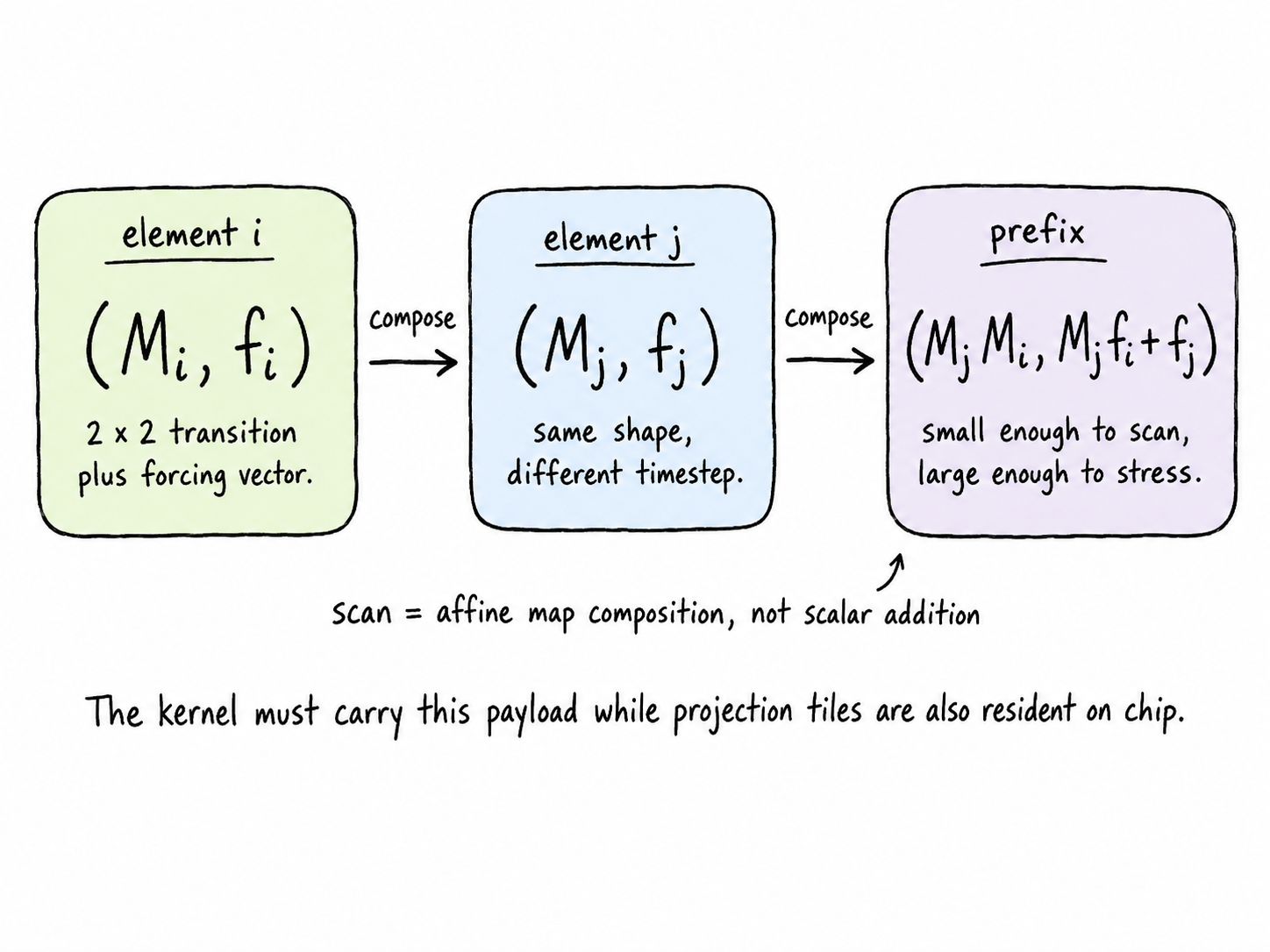
The recurrent update has serial semantics, but it is not necessarily trained serially. Linear recurrences can be parallelized through an associative scan, building on parallel-prefix primitives and their use in linear recurrent networks [5][6]. For a timestep-specific affine map
\[ s_{t+1} = M_t s_t + f_t, \]the scan element is the pair \((M_t, f_t)\). Two adjacent elements compose as
\[ (M_j, f_j) \star (M_i, f_i) = (M_j M_i,\; M_j f_i + f_j). \]This operation is associative, so a full sequence can be evaluated with logarithmic parallel depth. But it is not a scalar prefix sum: each element carries a transition object and a forcing vector. For oscillator models, that payload is small, but not free.
The associativity is easy to verify. Applying element i and then element j gives
So scans solve serialization, but do they solve performance? Not by themselves. In an IO-aware fused kernel, transition and forcing entries still occupy registers, shared memory, and compact global prefix records. The scan is algorithmically elegant, but the hardware still sees a payload that must be scheduled.
Part II
Block-Sparse Projection Scaling
Where Dense Projections Bite
Let \(L\) be sequence length, \(H\) the hidden width, and \(P\) the oscillator state size. The recurrence work scales like
\[ \text{recurrence work} = \Theta(LP), \]while the two dense projections scale like
\[ \text{projection work} = \Theta(LHP), \qquad \text{projection parameters} = \Theta(HP). \]This asymmetry creates a subtle failure mode. The oscillator recurrence is local and structured: each channel carries a small dynamical state with a spectral interpretation. The projections are global and dense: every hidden channel can actuate every oscillator, and every oscillator can be read by every hidden channel. As \(H\) and \(P\) grow, the dense actuator/sensor maps can dominate the cost, the parameter count, and the effective capacity of the layer.
A useful picture is a bank of resonators. The recurrence determines how each resonator rings; \(B\) is the actuator matrix; \(C\) is the sensor matrix. Dense \(B\) and \(C\) give every actuator access to every resonator and every sensor access to every resonator. That is flexible, but it can make the layer behave more like dense mixing wrapped around a cheap recurrent core.
That is not just an accounting issue. If the dense projections are too expressive, they can absorb much of the learning burden that should be carried by the recurrent dynamics. The model may still train, but the structured state-space part becomes less central. In harder regimes, this can also make optimization less stable because a large all-to-all projection system is being learned around a comparatively small and constrained recurrent mechanism.
This gets sharper in stacked architectures. With \(N_{\mathrm{blocks}}\) layers, the dense projection terms repeat at every block. If \(H\) and \(P\) grow together, \(HP\) is where parameters, FLOPs, and activation traffic accumulate.
The goal is not simply to make projections smaller. It is to control which projection couplings exist, so adding state capacity does not automatically create a fully dense hidden-state interaction at every timestep. Architectural sparsity is useful here because it is both a cost reduction and an inductive bias.
Block-Sparse Projections
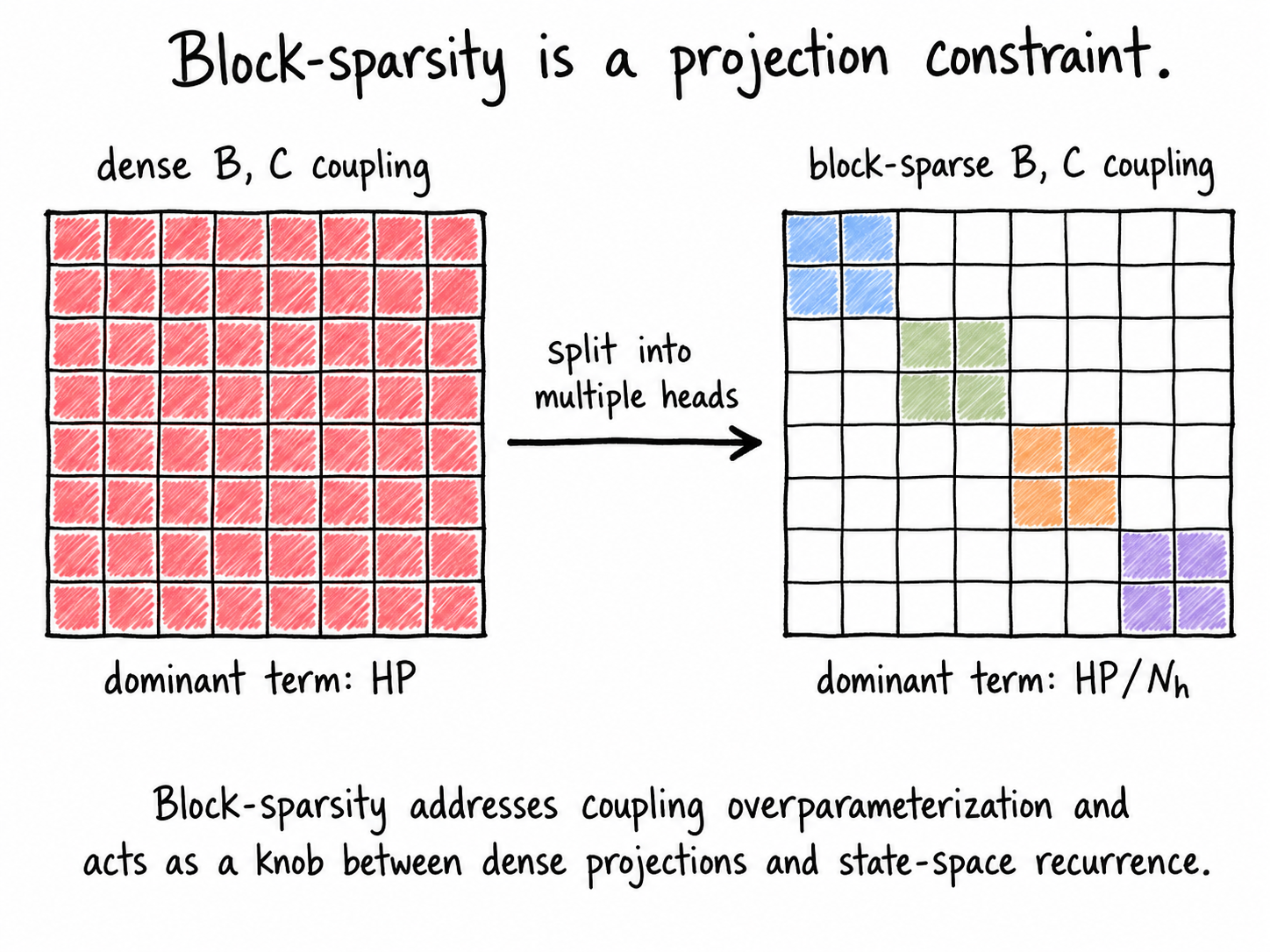
The block-sparse construction splits the hidden and state dimensions into \(N_h\) heads:
\[ H = N_h H_{\mathrm{head}}, \qquad P = N_h P_{\mathrm{head}}. \]Instead of dense \(B\) and \(C\), use block-diagonal projections:
\[ B_{\mathrm{MH}} = \operatorname{blockdiag}(B_1,\ldots,B_{N_h}), \qquad C_{\mathrm{MH}} = \operatorname{blockdiag}(C_1,\ldots,C_{N_h}). \]Each head gets a local hidden subspace and a local oscillator subspace. The recurrence inside each head is unchanged. Under a uniform partition, the dominant projection coupling drops from \(HP\) to \(HP/N_h\). The total oscillator budget \(P\) is preserved; what changes is which hidden channels are allowed to couple to which oscillator channels. The number of heads therefore becomes a knob: one head recovers dense projection coupling, while more heads impose stronger architectural sparsity.
More generally, for non-uniform heads with hidden sizes \(H_m\) and state sizes \(P_m\), the projection cost becomes
\[ \sum_{m=1}^{N_h} H_m P_m \]instead of \(HP\). Under uniform heads, \(H_m = H/N_h\) and \(P_m = P/N_h\), so
\[ \sum_{m=1}^{N_h} H_m P_m = N_h\left(\frac{H}{N_h}\right)\left(\frac{P}{N_h}\right) = \frac{HP}{N_h}. \]Since both \(B\) and \(C\) have this structure, the same reduction applies to the dominant input and output projection terms. The recurrence itself still sees the same total number of oscillator channels across all heads.
This is why the term "multi-head" is less important than the term "block-diagonal." The mathematical object is a structured sparsity pattern on the projection matrices. Separate heads process separate subspaces, and an optional output projection can remix the concatenated heads afterward. In that sense, the design is closer to controlled coupling than to compression: it decides where dense mixing is allowed to happen.
What does block-sparsity not do? It does not approximate the recurrence or prune oscillator channels. It simply prevents hidden features in head m from directly exciting oscillator states in head n inside \(B\) and \(C\). Cross-head communication can still happen through neighboring layers, residual paths, MLPs, normalization, or an explicit output projection.
The optional output projection is a deliberate tradeoff. Without it, the layer enforces head-local processing throughout the recurrent path. With it, each head first applies its own oscillator dynamics, and a dense hidden-space map then restores global channel mixing. The \(H^2\) term is not free, but it is applied after the recurrent state computation has already been split into head-local dynamical subspaces.
| Layer | Projection structure | Interpretation |
|---|---|---|
| Dense single head | \(HP\) coupling | Maximum mixing, but projections can dominate the recurrent structure. |
| Block-sparse heads | \(HP/N_h\) coupling | Separate oscillator subspaces with reduced dense coupling. |
| Heads + output projection | \(HP/N_h + H^2\) | Head-local recurrence followed by global channel remixing. |
Does Block-Sparsity Help?
Block-sparsity immediately changes the parameter count. That is useful, but it also makes the first empirical question harder: if a multi-headed model improves, is it because the block structure redistributes capacity better, or because the comparison accidentally changed the amount of capacity? The clean first test is therefore iso-parameter: match the parameter budget, then ask whether block-sparse projection structure itself helps.
More details.
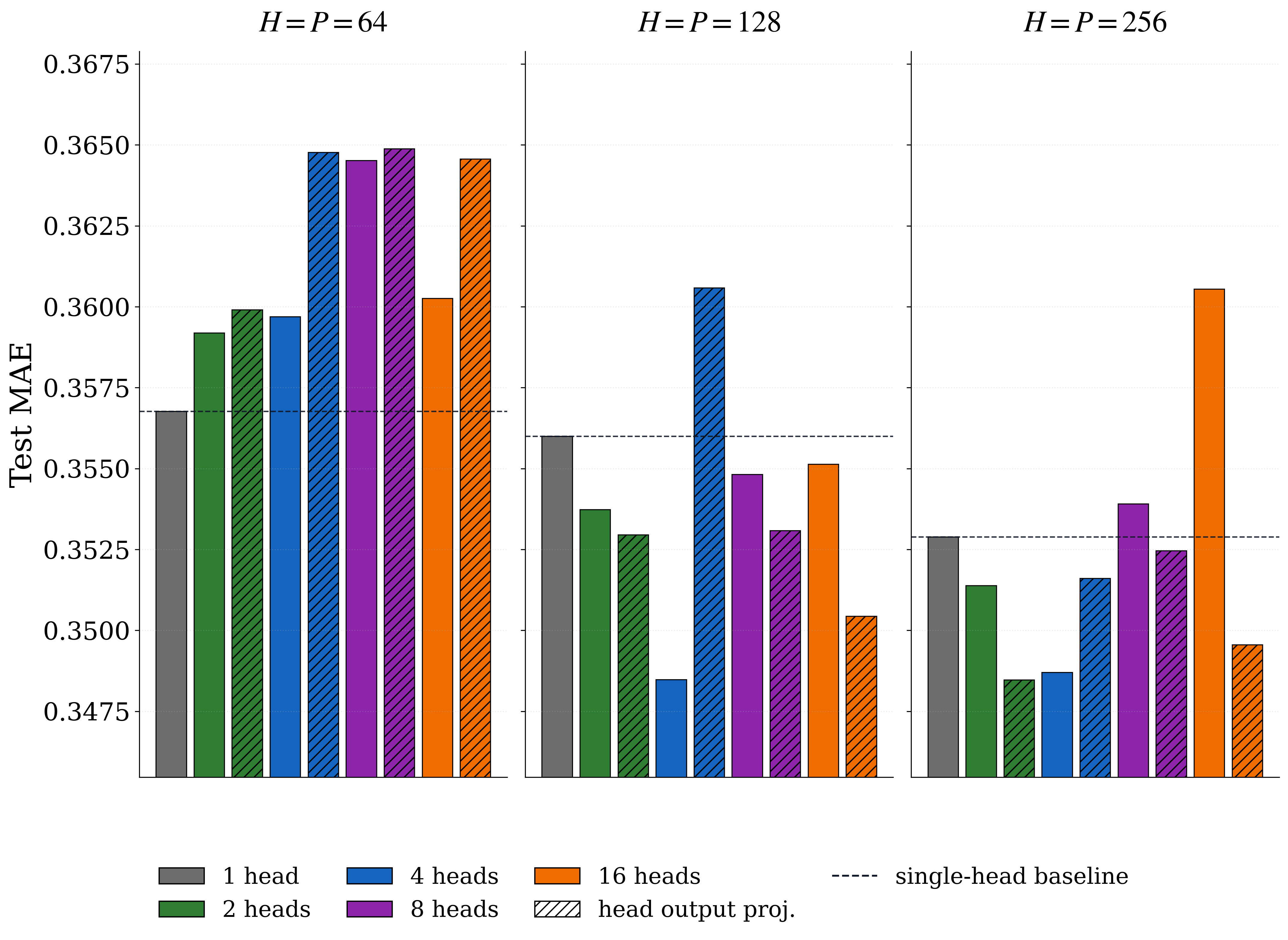
The iso-parameter comparison starts from a dense single-head baseline with fixed budget label \(H=P=d\). A same-width \(N_h\)-head version would automatically have fewer projection parameters, since the dominant dense coupling changes from \(HP\) to \(HP/N_h\). To isolate structure from parameter count, the multi-headed variants are widened until their total parameter count approximately matches the dense baseline budget.
The actual matching is done at the full model level, not only on the projection formula: the hidden/state dimensions of the MH variants are increased experimentally until the total trainable parameter count is as close as possible to the dense baseline, including surrounding pieces such as recurrent parameters, readouts, and GLU/MLP components. The main idea is that the MH model spends the saved dense-coupling budget on larger head-local representations.
The result is regime-dependent in exactly the way one would expect from a capacity-redistribution mechanism. At \(H=P=64\), the single-head baseline remained strongest. Splitting a small model into heads makes each head too narrow, so the sparsity constraint removes representation power before it removes a meaningful bottleneck. The extreme version would be \(H_{\mathrm{head}}=P_{\mathrm{head}}=1\): every head has a tiny local state and very little room to learn a useful sub-representation.
Once the dimensions are large enough, the story changes. At \(H=P=128\) and \(H=P=256\), the block-sparse variants were stronger, and the output projection often helped. This suggests that the heads need enough local capacity to specialize, after which the block structure becomes useful: each head learns its own oscillator subspace, and later layers or an output projection can combine the head outputs. This is conceptually similar to why multi-head attention is useful: the point is not only sparsity, but separately learned subspaces that can later be recombined.
The next question is the practical one: if we stop iso-parameter matching and let block-sparsity actually reduce projection parameters, can MH-DOSS still do better? In several benchmark groups, yes. The DOSS baseline is the damped oscillator framework of Boyer et al.; MH-DOSS keeps that recurrent core and applies the block-sparse projection structure around it. For the same total hidden/state budget, dense DOSS uses the dominant coupling \(HP\), while uniform \(N_h\)-head MH-DOSS uses \(HP/N_h\), before any optional output projection.
| Task | Benchmark / metric | DOSS | MH-DOSS |
|---|---|---|---|
| Classification | UEA average accuracy | 67.35% | 68.13% |
| Regression | PPG-DaLiA test MSE \(\times 10^{-2}\) | 5.74 | 5.69 |
| Forecasting | Average MSE | 0.977 | 0.846 |
More details.
The classification result averages six UEA multivariate time-series classification datasets: EigenWorms, SelfRegulationSCP1, SelfRegulationSCP2, EthanolConcentration, Heartbeat, and MotorImagery. These datasets cover biological motion, physiological signals, chemistry, cardiac dynamics, and motor-imagery EEG. The point of the aggregate row is not that every dataset behaves identically, but that MH-DOSS improved the DOSS row across this classification suite while reducing projection coupling.
The regression result is PPG-DaLiA, a long-sequence heart-rate estimation task from wearable photoplethysmography and motion signals. This is a useful stress test because the sequences can be very long, so both recurrent memory and implementation efficiency matter.
The forecasting result averages the hardest 720-step prediction setting across ETTh1, ETTh2, ETTm1, Weather, and Electricity. These are generic masked sequence-to-sequence forecasting evaluations rather than forecasting-specialized architectures. In this group, MH-DOSS is better on ETTh2, Weather, and Electricity, while DOSS is better on ETTh1 and ETTm1.
MH-DOSS is not better than DOSS on every individual dataset, but it performs better on average in these comparisons. That is the useful conclusion: when each head has enough local capacity, block-sparsity can reduce dense coupling, use fewer projection parameters, and still improve aggregate performance.
Why might this help? One explanation is coupling overparameterization. Dense \(B\) and \(C\) let every hidden channel interact with every oscillator channel, which can give the projection path too much responsibility. Block-sparsity forces different groups of channels to learn separate oscillator subspaces before the model remixes them. That can act like a regularizer, improve capacity allocation, and keep the recurrent dynamics from being overshadowed by dense input/output maps.
This is why the systems story pairs naturally with the modeling story. The model creates smaller independent projection-scan-projection problems; the IO-aware kernel turns those problems into hardware-friendly tiles.
Part III
IO-Aware Fused Kernels
Why Is It Still Slow?
Block-sparsity fixes one kind of inefficiency, but not all of it. Even after the projection matrices are head-local, a straightforward implementation still tends to express the layer as three separate tensor programs:
- project hidden activations into state-space matrices \(M,F\),
- scan those matrices over the sequence,
- project the scanned state-space result back to hidden space.
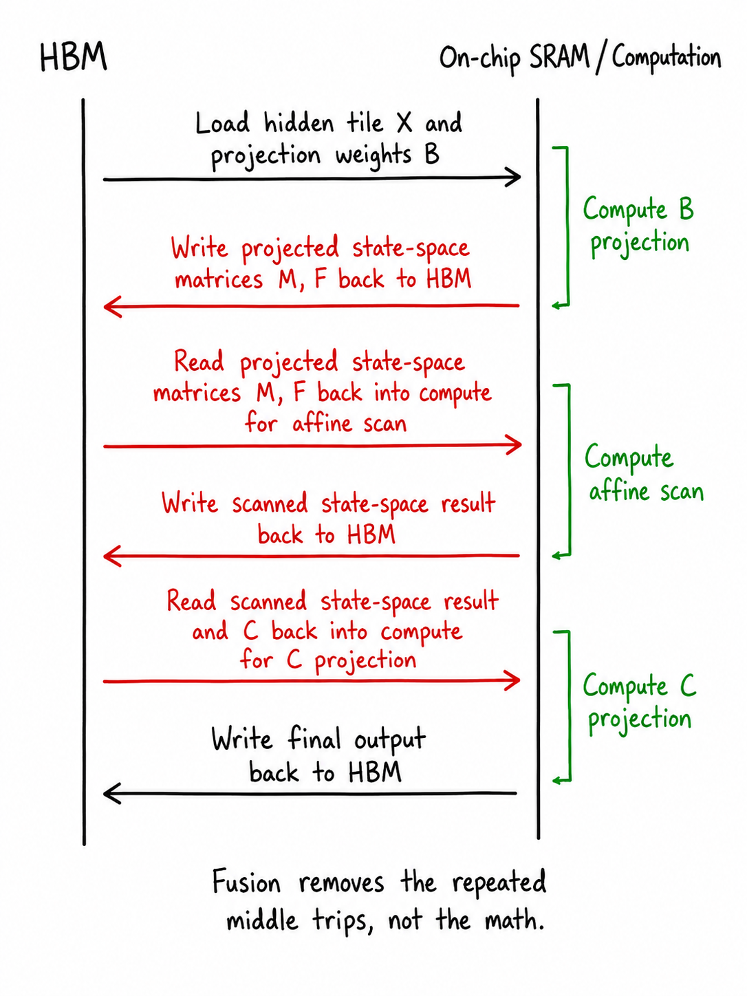
The issue is the handoff. The projected \(M,F\) values are not meaningful outputs; they exist so the scan can consume them. The scanned state-space result is similar; it exists so the \(C\)-projection can consume it. If these intermediates are written to HBM and then read back, the implementation is paying for a trip through global memory that the math never asked for.
This matters because the temporary state-domain tensors scale with \(LP\), while hidden activations scale with \(LH\). For long sequences and large state sizes, the intermediates can become some of the largest objects in the layer, despite having a lifetime of exactly one neighboring operation.
A representative packed forward implementation can have state-space peak memory on the order of
\[ 72LP + 12LH \quad \text{bytes} \]for one sequence and one layer, before neighboring MLP/GLU activations. The constants depend on layout and precision, but the lesson is stable: the \(LP\) intermediates are the memory problem. The kernel question is therefore simple: can we keep those middle values on chip?
Can We Keep the Middle On Chip?
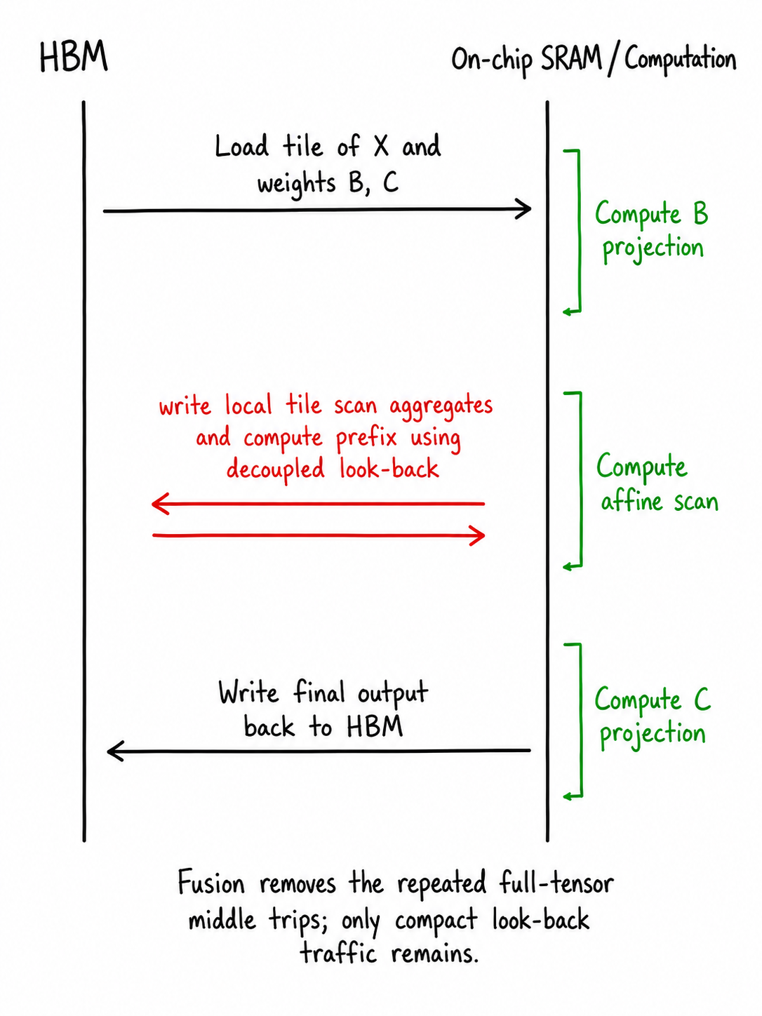
FlashDOSS answers yes by changing the schedule, not the layer. The mathematical path is still
\[ \text{\(B\)-projection} \;\longrightarrow\; \text{affine scan} \;\longrightarrow\; \text{\(C\)-projection}. \]but the execution becomes a head-local pipeline. A thread block loads a sequence tile, a state tile, projection weights, and oscillator parameters. It computes projected \(M,F\) values into an on-chip buffer, scans the tile, stitches in the prefix from previous sequence tiles, and immediately feeds the scanned result into the \(C\)-projection. The middle tensors are produced and consumed before they become global tensors.
This is a small wording difference with a large systems consequence. "Fuse three kernels" is not the real objective. The real objective is to preserve producer-consumer locality: \(B\) produces what scan needs, scan produces what \(C\) needs, and the implementation should not turn those handoffs into HBM traffic.
The head-local structure from MH-DOSS is what makes this clean. One tile can focus on one batch element, one head, a chunk of sequence, and a slice of oscillator state. Within that tile, the kernel stages the hidden inputs, oscillator parameters, projection weights, scan payload, and output accumulator without needing dense cross-head communication.
The awkward part is that the pieces want different shapes. The projections want GEMM-friendly Tensor Core tiles. The scan wants a prefix order over timesteps and carries an affine oscillator payload. FlashDOSS has to make those two worlds share one tile.
The algorithm separates unavoidable movement from avoidable movement. Inputs, weights, oscillator parameters, final outputs, and compact prefix records still cross memory boundaries. Projected state-space matrices and scanned state-space results do not need to become global tensors.
There is also a scan-specific complication hidden inside the word "prefix." This is not scalar addition. Each timestep carries a small affine map: transition entries for an oscillator block plus state-space contributions. Those objects are compact compared with a full \(L\times P\) state tensor, but they are large enough that register pressure and tile shape matter.
Within a sequence tile, warp-level prefix operations move these payloads across timesteps. That keeps the local scan fast, but it also turns scan design into resource budgeting: every extra payload entry competes with projection fragments and shared-memory buffers.
This is where the analogy to FlashAttention is useful [7]. FlashAttention avoids materializing the attention matrix. FlashDOSS avoids materializing projected state-space matrices and scanned state-space results. In both cases, the speedup comes from changing where intermediate values live, not from changing the math.
But the dependency is different. Attention tiles need online normalization statistics and value accumulation. FlashDOSS tiles need prefix information across the sequence: tile 7 depends on the aggregate effect of tiles 0 through 6. That is the one thing that prevents the fused kernel from being a simple tiled GEMM pipeline.
How Do Tiles Know Their Prefix?
A sequence tile can scan locally, but it does not know the correct global scanned state until it knows the prefix from all earlier tiles. The conventional solution is staged:
- run local scans and write tile aggregates,
- scan the tile aggregates in another kernel,
- launch a fix-up kernel to apply prefixes to every tile.
That works, but it breaks the story. The kernel would have to stop after the local scan, write a state-sized object, wait for another kernel to compute prefixes, and then replay the result. FlashDOSS needs a single-stage scan so the same kernel can project, scan, prefix-correct, and project back without committing the large state tensor to HBM.
Decoupled look-back gives that single-stage path [8]. Each tile scans locally, publishes a compact aggregate, and then looks backward through aggregate/prefix records. If it finds a ready prefix, it stops. If it finds only aggregates, it combines them and keeps looking back. The kernel may redo a small amount of summary work, but it avoids another global pass over the full state tensor.
The trick is separating aggregates from prefixes. An aggregate is the effect of one tile alone. A prefix is the effect of all previous tiles up to a point. Once tile k knows its prefix, later tiles can stop looking back as soon as they see it.
That is the "decoupled" part: local scan work proceeds before the complete global prefix is known. The redundant work recomposes compact summaries, not full tensors.
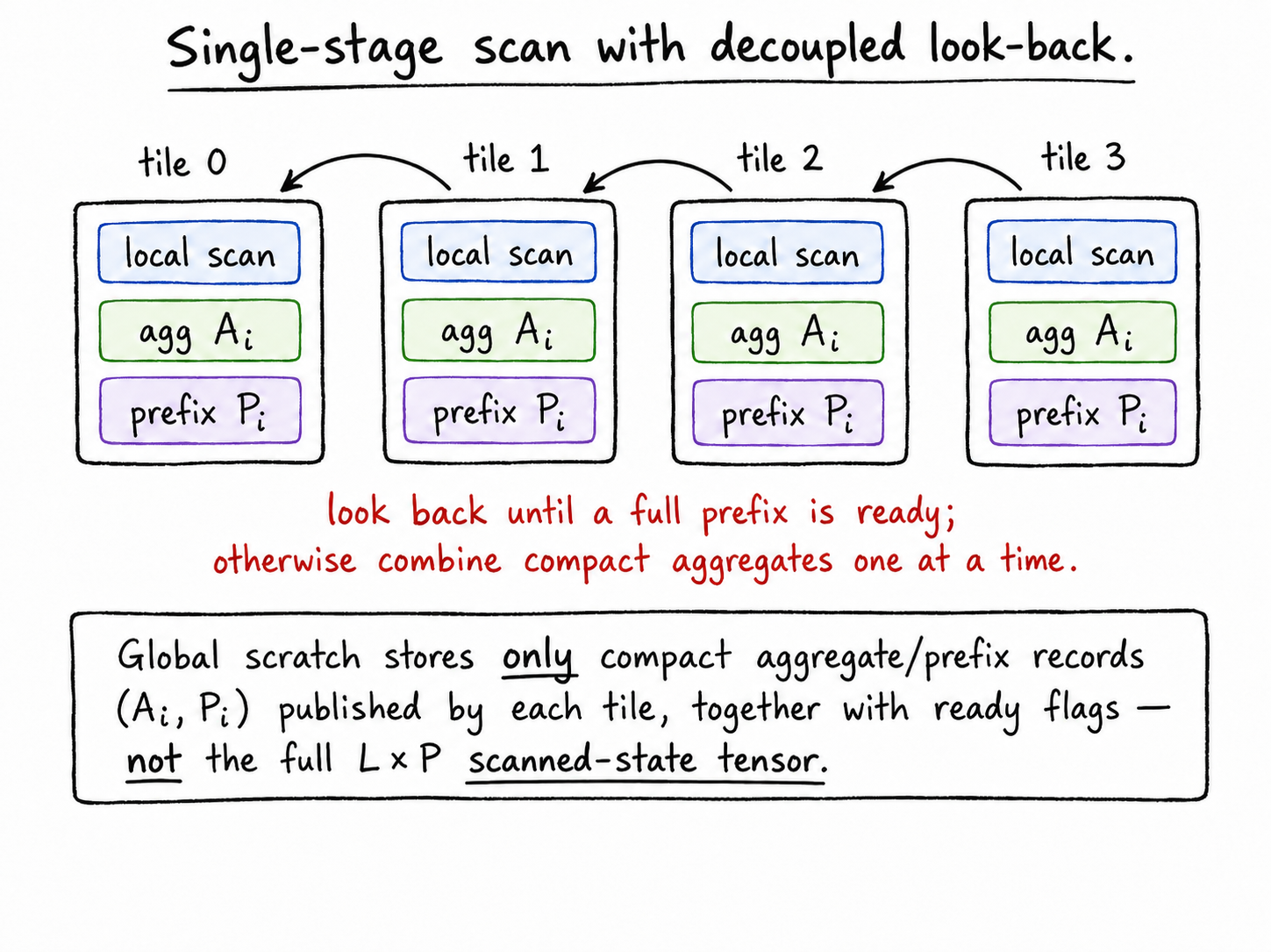
In implementation terms, each tile publishes an aggregate and, later, a prefix. Ready flags tell later tiles which records are safe to consume. These records contain the affine oscillator payload, so they are compact compared with the full \(L\times P\) scanned-state tensor.
This is the key systems link: decoupled look-back keeps prefix propagation inside the fused execution. Once a tile corrects its local scan, it can proceed directly to the \(C\)-projection.
The remaining engineering tension is tile shape. The \(B\) and \(C\) projections want GEMM-friendly Tensor Core tiles, while the scan carries an affine oscillator payload through registers and shared memory. Larger state tiles improve projection arithmetic intensity but increase scan payload pressure; longer sequence tiles amortize prefix overhead but store more local scan state. This is why head-locality matters: block-sparse heads are not only a modeling structure, but also a natural unit for fused execution.
Did It Pay Off?
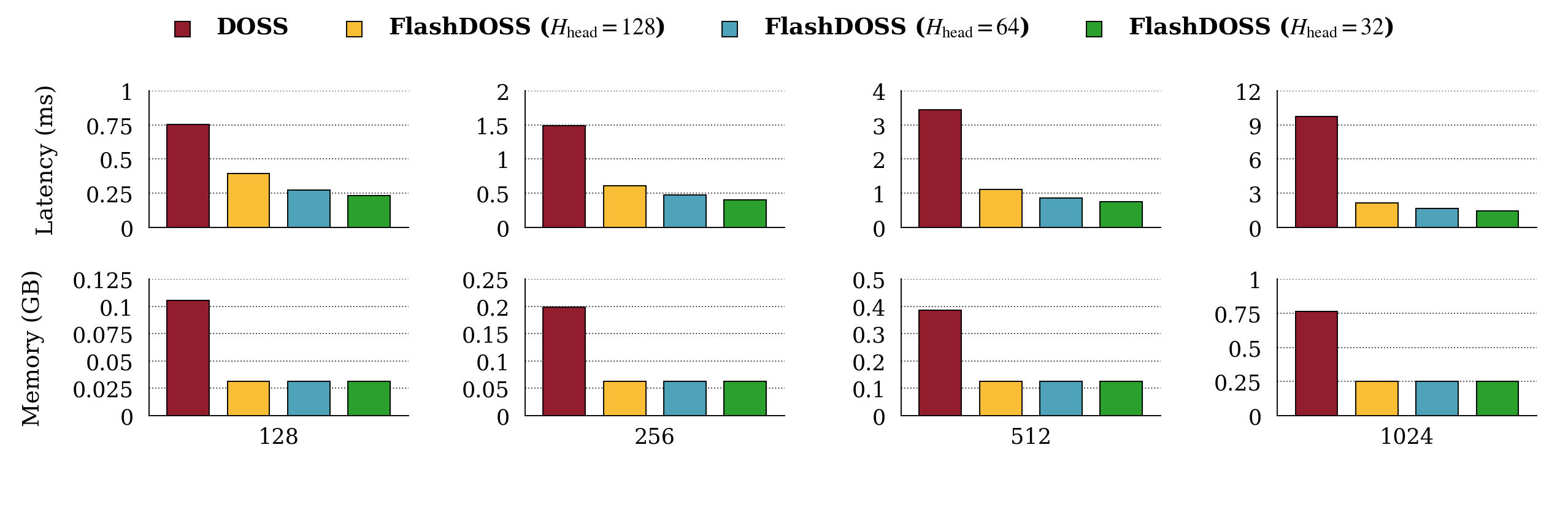
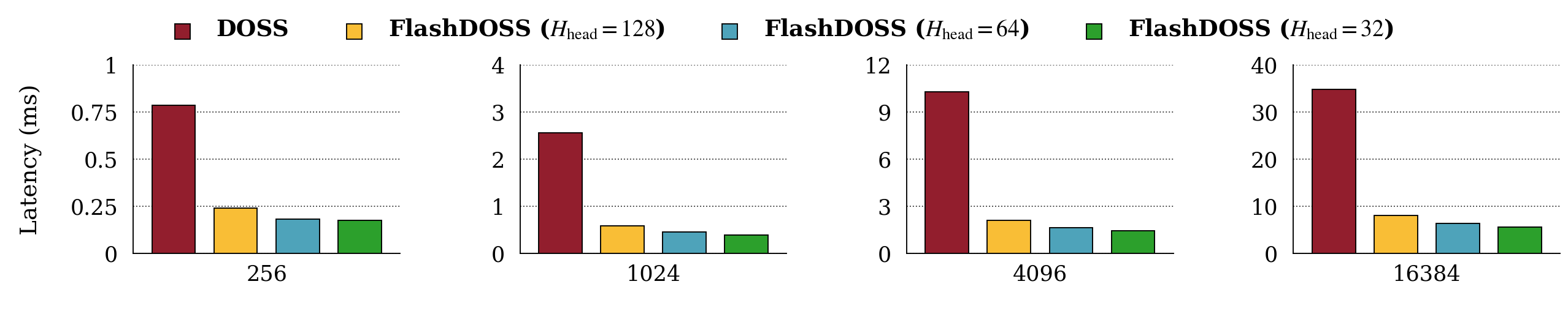
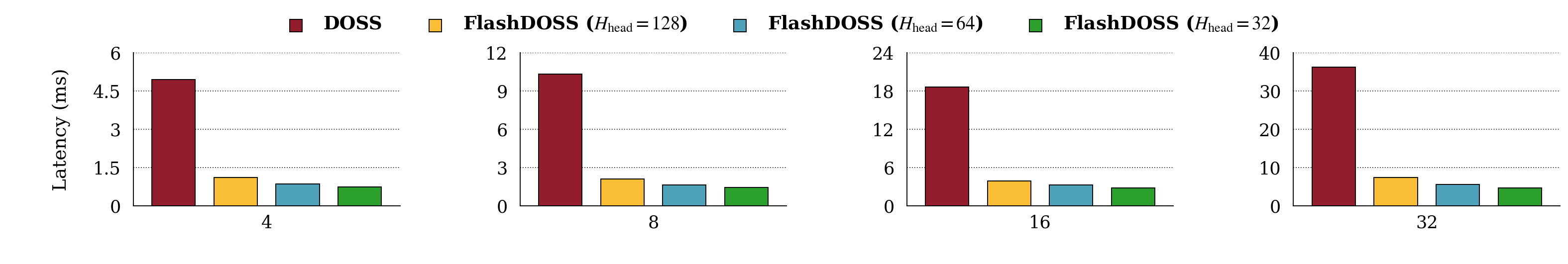
On an NVIDIA A100, the IO-aware implementation reduced layer-level runtime and peak memory in the regimes where the memory story predicts it should matter.
The dimension sweep is the cleanest systems stress test because it increases \(H\) and \(P\) together, exactly where dense projection work and state-domain materialization grow quickly. The IO-aware implementation is strongest when per-head tile sizes keep the projections efficient without making the scan payload too large.
| Measurement | Observed result | Scope |
|---|---|---|
| Main dimension sweep | up to 6.8x lower runtime | layer-level forward benchmark |
| All sweeps | up to 7.8x lower runtime | largest speedup in batch-size sweep |
| Memory | about 3x lower peak allocation | layer-level memory footprint |
The memory result is as important as the latency result. It confirms the intended mechanism: the kernel is not merely faster because it is lower overhead; it is faster because it avoids allocating and retaining the large state-domain intermediates.
These are layer-level forward benchmarks, not full training-pipeline acceleration. End-to-end training includes optimizer overhead, MLP/GLU blocks, normalization, backward passes, and framework overhead. The narrower point is still useful: for the state-space layer itself, the IO-aware fused path removes a real bottleneck.
Closing
The Takeaway
The final design is not just "make the model sparse" and not just "write a faster kernel." The two pieces solve different versions of the same scaling problem. Block-sparse heads decide where capacity is allowed to couple. The IO-aware kernel decides where intermediates are allowed to live.
That is the broader lesson: efficient sequence models need the math, parameterization, and hardware schedule to agree. A recurrence can be linear-time and still be slow. A projection can be expressive and still be too dense. A scan can be parallel and still be memory-bound.
This gives a useful test for future SSM designs: where does the capacity live, where do the intermediates live, and can the GPU execute the layer without unnecessary traffic? If any one of those answers is awkward, the theoretical advantage may not survive contact with real hardware.
When the pieces do align, a modeling choice becomes a systems advantage. Head-local oscillator subspaces reduce projection coupling, define smaller projection/scan tiles, and fit naturally into a fused pipeline. Decoupled look-back keeps the scan single-stage. The point is not sparsity for its own sake or kernels for their own sake, but making the architecture and execution plan pull in the same direction.
References
- Ashish Vaswani, Noam Shazeer, Niki Parmar, Jakob Uszkoreit, Llion Jones, Aidan N. Gomez, Lukasz Kaiser, and Illia Polosukhin. Attention Is All You Need. NeurIPS, 2017.
- Albert Gu, Karan Goel, and Christopher Re. Efficiently Modeling Long Sequences with Structured State Spaces. ICLR, 2022.
- T. Konstantin Rusch and Daniela Rus. Oscillatory State-Space Models. ICLR, 2025.
- Jared Boyer, T. Konstantin Rusch, and Daniela Rus. Learning to Dissipate Energy in Oscillatory State-Space Models. arXiv, 2025.
- Guy E. Blelloch. Prefix Sums and Their Applications. Technical Report CMU-CS-90-190, Carnegie Mellon University, 1990.
- Eric Martin and Christopher Cundy. Parallelizing Linear Recurrent Neural Nets Over Sequence Length. ICLR, 2018.
- Tri Dao, Daniel Y. Fu, Stefano Ermon, Atri Rudra, and Christopher Re. FlashAttention: Fast and Memory-Efficient Exact Attention with IO-Awareness. NeurIPS, 2022.
- Duane Merrill and Michael Garland. Single-pass Parallel Prefix Scan with Decoupled Look-back. NVIDIA Technical Report NVR-2016-002, 2016.